一.探索样本间关系 1.样本相关性分析 1 2 3 4 5 6 7 8 9 10 11 12 13 14 15 16 17 18 19 20 21 22 23 24 25 26 27 > head(dds) class: DESeqDataSet dim: 6 4 metadata(1 ): version assays(1 ): counts rownames(6 ): ENSG00000000003 ENSG00000000005 ... ENSG00000000460 ENSG00000000938 rowData names(0 ): colnames(4 ): control1 control2 treat1 treat2 colData names(1 ): condition > as_dds<-assay(dds) > head(as_dds) control1 control2 treat1 treat2 ENSG00000000003 796 349 780 937 ENSG00000000005 0 0 0 1 ENSG00000000419 389 174 403 503 ENSG00000000457 288 108 218 283 ENSG00000000460 506 208 451 543 ENSG00000000938 0 0 0 0 > sample_cor <- cor(as_dds,method = 'pearson' ) > head(sample_cor) control1 control2 treat1 treat2 control1 1.0000000 0.9952493 0.9397933 0.9937118 control2 0.9952493 1.0000000 0.9090246 0.9824907 treat1 0.9397933 0.9090246 1.0000000 0.9657993 treat2 0.9937118 0.9824907 0.9657993 1.0000000 pheatmap(sample_cor)
2.样本聚类分析 1 2 3 distance<-dist(t(as_dds) sample_hc <- hclust(distance) plot(sample_hc)
二.PCA分析 进行PCA之前是要进行归一化的,因为在降维映射的过程中, 存在映射误差, 所有在对高维特征降维之前, 需要做特征归一化(feature normalization), 这个归一化操作包括: (1) feature scaling (让所有的特征拥有相似的尺度, 要不然一个特征特别小, 一个特征特别大会影响降维的效果) (2) zero mean normalization (零均值归一化)。
1 2 rlog() may take a few minutes with 30 or more samples, vst() is a much faster transformation
官方就会建议样本量大于30的时候用vst.
intgroup:分组
官方解释:interesting groups: a character vector of names in colData(x) to use for grouping。也就是在构建dds的时候的分组,实际上这个分组最后影响的是PCA图中的颜色,但是并不影响PCA图中各个样本的位置。换句话说,PCA降维的是时候并不会考虑这个分组。
1 2 3 4 5 6 7 8 9 10 11 12 13 14 15 16 17 vsd <- rlog(dds, blind = FALSE ) pcaData <- plotPCA(vsd, intgroup="condition" , returnData=TRUE ) > pcaData PC1 PC2 group condition name control1 -4.09219210 0.3231349 control control control1 control2 -5.60305114 0.8966271 control control control2 treat1 9.77130695 0.6350322 treat treat treat1 treat2 -0.07606371 -1.8547942 treat treat treat2 percentVar <- round(100 * attr(pcaData, "percentVar" )) ggplot(pcaData, aes(PC1, PC2, color=condition)) + geom_point(size=3 ) + xlab(paste0("PC1: " ,percentVar[1 ],"% variance" )) + ylab(paste0("PC2: " ,percentVar[2 ],"% variance" )) + coord_fixed()
二.火山图 火山图能反应组间基因表达情况(理论上来说应该用padj,但是这个例子用padj画图不好看)
1.利用EnhancedVolcano包 1 2 3 4 5 6 7 8 9 10 11 12 volcanoplot<-EnhancedVolcano(res, lab = rownames(res), x = 'log2FoldChange' , y = 'pvalue' , xlim = c(-5 ,5 ), ylim = c(0 ,10 ), pCutoff = 10e-5 , FCcutoff = 1 , col=c('black' , 'blue' , 'green' , 'red3' ), colAlpha = 1 , title = 'control vs treat' ) ggsave("volcanoplot.png" ,volcanolot)
2.利用ggplot2画图 1 2 3 4 5 6 7 8 9 10 11 12 13 14 15 16 17 18 19 20 21 22 23 24 25 26 data <- data.frame(gene = row.names(res), pvalue= res$pvalue, log2FoldChange = res$log2FoldChange) data <- na.omit(data) data <- mutate(data, color = case_when(data$log2FoldChange > 1 & data$pvalue<0.05 ~ "Increased" , data$log2FoldChange < 1 & data$pvalue< 0.05 ~ "Decreased" , data$pvalue>0.05 ~ "nonsignificant" )) my_palette <- c('#E64B35FF' , '#4DBBD5FF' ,'#999999' ) library (ggplot2)ggplot(data = data, aes(x = log2FoldChange, y = -log10(pvalue))) + geom_point(aes(color =color, size = abs(log2FoldChange))) + geom_hline(yintercept = -log10(0.05 ), linetype = 'dashed' ) + geom_vline(xintercept = c(-1 , 1 ), linetype = 'dashed' ) + scale_color_manual(values = my_palette) + scale_size(range = c(0.1 , 3 )) + xlim(-5 ,5 )+ylim(0 ,10 )+ theme_bw()
3.热图(挑取差异表达前30的基因画图) 1 2 3 4 5 6 7 8 9 10 11 12 13 14 15 16 17 18 19 20 21 22 23 24 25 26 27 28 29 30 31 32 33 34 35 36 37 38 39 40 41 42 43 44 45 46 47 48 49 50 51 52 53 54 55 56 57 58 59 60 61 62 63 64 65 66 67 68 69 70 71 72 73 74 75 76 77 78 79 80 81 82 83 84 85 > top_30_gene <-arrange(diff_name,desc(abs(log2FoldChange)))[1 :30 ,] > head(top_30_gene) ensembl_gene_id baseMean log2FoldChange lfcSE stat 1 ENSG00000178691 531.5924 2.899835 0.2360647 12.284069 2 ENSG00000172239 238.1623 1.311505 0.2546097 5.151041 3 ENSG00000164172 256.8816 1.281828 0.2427446 5.280562 4 ENSG00000187772 730.2692 1.256584 0.2550770 4.926295 5 ENSG00000163376 165.2589 1.248009 0.3180561 3.923863 6 ENSG00000128512 181.1727 1.236845 0.2955839 4.184413 pvalue padj hgnc_symbol chromosome_name 1 1.103076e-34 9.164356e-31 SUZ12 17 2 2.590440e-07 3.074482e-04 PAIP1 5 3 1.287882e-07 2.139944e-04 MOCS2 5 4 8.380340e-07 8.702983e-04 LIN28B 6 5 8.714023e-05 2.895844e-02 KBTBD8 3 6 2.859045e-05 1.250155e-02 DOCK4 7 start_position end_position band 1 31937007 32001038 q11.22 43526267 43557758 p123 53095679 53110063 q11.24 104936616 105083332 q16.35 66998307 67011210 p14.16 111726110 112206407 q31.1> head(as_dds) control1 control2 treat1 treat2 ENSG00000000003 796 349 780 937 ENSG00000000005 0 0 0 1 ENSG00000000419 389 174 403 503 ENSG00000000457 288 108 218 283 ENSG00000000460 506 208 451 543 ENSG00000000938 0 0 0 0 > as_dds2 <- rownames_to_column(as_dds,var='ensembl_gene_id' ) Error in rownames_to_column(as_dds, var = "ensembl_gene_id" ) : is.data.frame(df) is not TRUE > as_dds2 <- rownames_to_column(as.data.frame(as_dds),var='ensembl_gene_id' ) > head(as_dds2) ensembl_gene_id control1 control2 treat1 treat2 1 ENSG00000000003 796 349 780 937 2 ENSG00000000005 0 0 0 1 3 ENSG00000000419 389 174 403 503 4 ENSG00000000457 288 108 218 283 5 ENSG00000000460 506 208 451 543 6 ENSG00000000938 0 0 0 0 > top_30_gene <- left_join(top_30_gene,as_dds2,by='ensembl_gene_id' ) > head(top_30_gene) ensembl_gene_id baseMean log2FoldChange lfcSE stat 1 ENSG00000178691 531.5924 2.899835 0.2360647 12.284069 2 ENSG00000172239 238.1623 1.311505 0.2546097 5.151041 3 ENSG00000164172 256.8816 1.281828 0.2427446 5.280562 4 ENSG00000187772 730.2692 1.256584 0.2550770 4.926295 5 ENSG00000163376 165.2589 1.248009 0.3180561 3.923863 6 ENSG00000128512 181.1727 1.236845 0.2955839 4.184413 pvalue padj hgnc_symbol chromosome_name 1 1.103076e-34 9.164356e-31 SUZ12 17 2 2.590440e-07 3.074482e-04 PAIP1 5 3 1.287882e-07 2.139944e-04 MOCS2 5 4 8.380340e-07 8.702983e-04 LIN28B 6 5 8.714023e-05 2.895844e-02 KBTBD8 3 6 2.859045e-05 1.250155e-02 DOCK4 7 start_position end_position band control1 control2 treat1 treat2 1 31937007 32001038 q11.2 1080 494 118 218 2 43526267 43557758 p12 348 198 165 193 3 53095679 53110063 q11.2 417 193 161 236 4 104936616 105083332 q16.3 1162 553 365 799 5 66998307 67011210 p14.1 245 133 83 180 6 111726110 112206407 q31.1 278 141 98 191 > pheatmap_data <- select(top_30_gene,'hgnc_symbol' ,'control1' ,'control2' ,'treat1' ,'treat2' ) > head(pheatmap_data) hgnc_symbol control1 control2 treat1 treat2 1 SUZ12 1080 494 118 218 2 PAIP1 348 198 165 193 3 MOCS2 417 193 161 236 4 LIN28B 1162 553 365 799 5 KBTBD8 245 133 83 180 6 DOCK4 278 141 98 191 > pheatmap_data <- column_to_rownames(pheatmap_data,var='hgnc_symbol' ) > head(pheatmap_data) control1 control2 treat1 treat2 SUZ12 1080 494 118 218 PAIP1 348 198 165 193 MOCS2 417 193 161 236 LIN28B 1162 553 365 799 KBTBD8 245 133 83 180 DOCK4 278 141 98 191
4.GO富集分析 理论应该使用deseq2筛选后得到的差异基因进行go,kegg富集分析;但是因为这个数据得到差异基因太少画图不好看,不一定能富集到通路,就用未筛选前的基因(所有基因)。
1.ID转换
1 2 3 4 5 6 7 8 9 10 11 12 13 14 15 16 17 18 19 20 21 22 BiocManager::install('org.Hs.eg.db' ) library ('org.Hs.eg.db' )library ('clusterProfiler' )all_gene<-as.data.frame(res) raw_count_table<-rownames_to_column(all_gene,var='ensembl_gene_id' ) gene <- raw_count_table$ensembl_gene_id > head(gene) [1 ] "ENSG00000000003" "ENSG00000000005" "ENSG00000000419" [4 ] "ENSG00000000457" "ENSG00000000460" "ENSG00000000938" gene.df <- bitr(gene,fromType = "ENSEMBL" , toType = c('SYMBOL' ,'ENTREZID' ), OrgDb = org.Hs.eg.db) > head(gene.df) ENSEMBL SYMBOL ENTREZID 1 ENSG00000000003 TSPAN6 7105 2 ENSG00000000005 TNMD 64102 3 ENSG00000000419 DPM1 8813 4 ENSG00000000457 SCYL3 57147 5 ENSG00000000460 C1orf112 55732 6 ENSG00000000938 FGR 2268
2.GO_CC富集
1 2 3 4 5 6 7 8 9 ego_cc <- enrichGO(gene=gene.df$ENSEMBL, OrgDb = org.Hs.eg.db, keyType = 'ENSEMBL' , ont = 'CC' , pAdjustMethod = 'BH' , pvalueCutoff = 0.01 , qvalueCutoff = 0.05 ) barplot(ego_cc,showCategory=18 ,title = 'The GO_CC ecnrichment analysis of all DEGS' )+ scale_size(range = c(2 ,12 ))+scale_x_discrete(labels=function (ego_cc) str_wrap(ego_cc,width = 25 ))
3.GO_BP富集
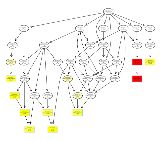
1 2 3 4 5 6 7 8 9 10 ego_bp<-enrichGO(gene = gene.df$ENSEMBL, OrgDb = org.Mm.eg.db, keyType = 'ENSEMBL' , ont = "BP" , pAdjustMethod = "BH" , pvalueCutoff = 0.01 , qvalueCutoff = 0.05 ) barplot(ego_bp,showCategory = 18 ,title="The GO_BP enrichment analysis of all DEGs " )+ scale_size(range=c(2 , 12 ))+ scale_x_discrete(labels=function (ego_bp) str_wrap(ego_bp,width = 25 ))
4.功能富集气泡图及go图
1 dotplot(ego_bp,font.size=10 )
5.KEGG富集分析 理论应该使用deseq2筛选后得到的差异基因进行go,kegg富集分析;但是因为这个数据得到差异基因太少(只有32个)画图不好看,不一定能富集到通路,就用未筛选前的基因(所有基因)。
1 2 3 4 5 6 enrich_kegg <- enrichKEGG(gene = gene.df$ENTREZID, organism = 'hsa' , pvalueCutoff = 0.1 ) head(enrich_kegg) barplot(enrich_kegg,showCategory=18 ,title = 'The KEGG ecnrichment analysis of all DEGS' )+ scale_size(range = c(2 ,12 ))+scale_x_discrete(labels=function (enrich_kegg) str_wrap(enrich_kegg,width = 25 ))
6.GSEA富集分析 该分析数据为deseq2经筛选后的差异基因(padj<0.05 & (log2FoldChange<-1 | log2FoldChange>1)
1 2 3 4 5 6 7 8 9 10 11 12 13 14 15 16 17 18 19 20 21 22 23 24 25 > gsea_gene_list <- diff_name$log2FoldChange > head(gsea_gene_list) [1 ] 0.9650973 0.7833167 -1.0576105 0.9222084 -0.6617466 0.8949043 > names(gsea_gene_list) <- diff_name$ensembl_gene_id > head(gsea_gene_list) ENSG00000039319 ENSG00000054598 ENSG00000064666 ENSG00000071794 0.9650973 0.7833167 -1.0576105 0.9222084 ENSG00000075624 ENSG00000077549 -0.6617466 0.8949043 > gsea_gene_list <- sort(gsea_gene_list,decreasing = TRUE ) > gsemf <- gseGO(gsea_gene_list,OrgDb = org.Hs.eg.db,keyType = 'ENSEMBL' ,pvalueCutoff = 1 ,ont = 'BP' ) preparing geneSet collections... GSEA analysis... leading edge analysis... done... > head(gsemf,1 ) ID Description setSize GO:0051716 GO:0051716 cellular response to stimulus 16 enrichmentScore NES pvalue p.adjust qvalues GO:0051716 -0.4359466 -1.588738 0.04227305 0.5428165 0.5428165 rank leading_edge GO:0051716 17 tags=75 %, list=53 %, signal=70 % core_enrichment GO:0051716 ENSG00000149311/ENSG00000039319/ENSG00000156650/ENSG00000117335/ENSG00000198887/ENSG00000158290/ENSG00000114978/ENSG00000054598/ENSG00000162521/ENSG00000075624/ENSG00000184009/ENSG00000064666 gseaplot(gsemf,geneSetID = 'GO:0051716' )
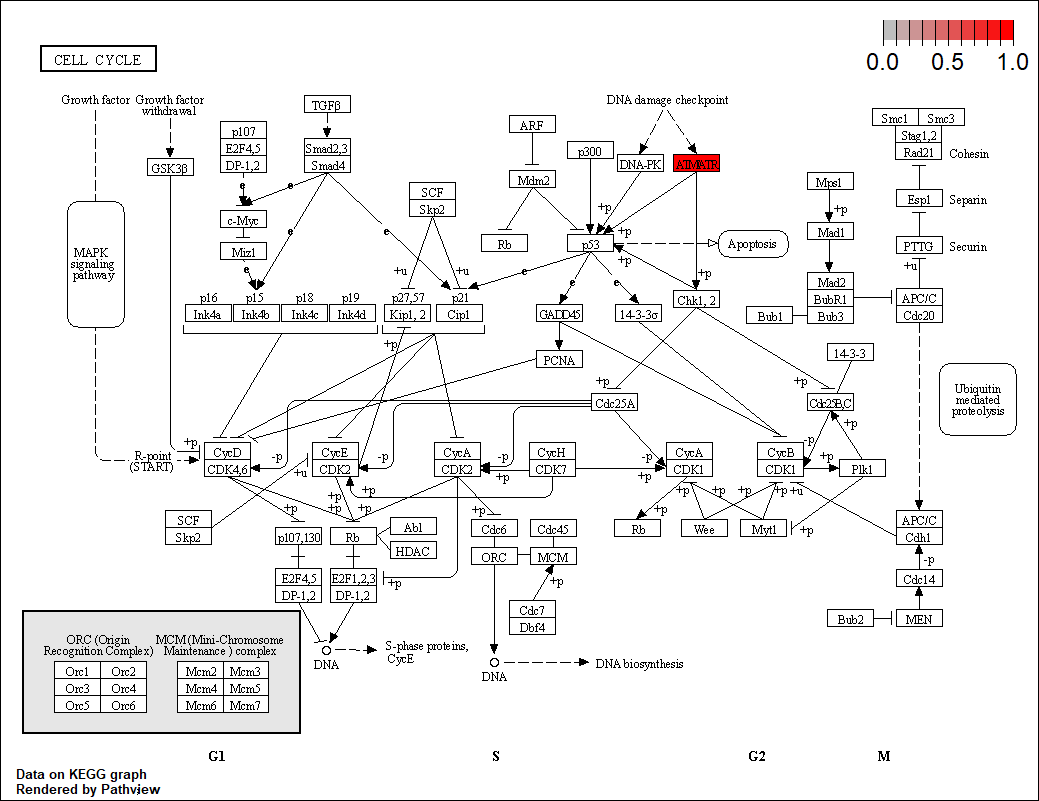
7.基因通路图 该分析数据为deseq2经筛选后的差异基因(padj<0.05 & (log2FoldChange<-1 | log2FoldChange>1),该数据得到的差异基因太少了,画图不好看。
1 2 3 4 5 6 7 8 9 10 11 12 13 14 15 16 17 18 19 20 21 22 23 24 25 26 27 28 29 30 31 32 33 34 35 36 37 38 39 40 41 42 43 44 45 46 47 48 49 50 51 52 53 54 55 56 57 58 > > head(diff_name) ensembl_gene_id baseMean log2FoldChange lfcSE stat pvalue padj 1 ENSG00000039319 522.7108 0.9650973 0.2447603 3.943030 8.045870e-05 0.028304572 2 ENSG00000054598 1253.0761 0.7833167 0.1776648 4.408959 1.038687e-05 0.005393382 3 ENSG00000064666 233.3811 -1.0576105 0.2623787 -4.030855 5.557431e-05 0.020986881 4 ENSG00000071794 1030.8820 0.9222084 0.2203282 4.185612 2.843993e-05 0.012501549 5 ENSG00000075624 7955.8749 -0.6617466 0.1679916 -3.939165 8.176573e-05 0.028304572 6 ENSG00000077549 598.6919 0.8949043 0.2002158 4.469698 7.833019e-06 0.004419020 hgnc_symbol chromosome_name start_position end_position band 1 ZFYVE16 5 80408013 80483379 q14.12 FOXC1 6 1609915 1613897 p25.33 CNN2 19 1026586 1039068 p13.34 HLTF 3 149030127 149086554 q245 ACTB 7 5526409 5563902 p22.16 CAPZB 1 19338775 19485539 p36.13> gene <- diff_name$ensembl_gene_id > path_gene.df <- bitr(gene,fromType = "ENSEMBL" , + toType = c('SYMBOL' ,'ENTREZID' ), + OrgDb = org.Hs.eg.db) > head(path_gene.df) ENSEMBL SYMBOL ENTREZID 1 ENSG00000039319 ZFYVE16 9765 2 ENSG00000054598 FOXC1 2296 3 ENSG00000064666 CNN2 1265 4 ENSG00000071794 HLTF 6596 5 ENSG00000075624 ACTB 60 6 ENSG00000077549 CAPZB 832 > path_gene.df <- merge(diff_name,path_gene.df,by.x='ensembl_gene_id' ,by.y='ENSEMBL' ) > head(path_gene.df) ensembl_gene_id baseMean log2FoldChange lfcSE stat pvalue padj 1 ENSG00000039319 522.7108 0.9650973 0.2447603 3.943030 8.045870e-05 0.028304572 2 ENSG00000054598 1253.0761 0.7833167 0.1776648 4.408959 1.038687e-05 0.005393382 3 ENSG00000064666 233.3811 -1.0576105 0.2623787 -4.030855 5.557431e-05 0.020986881 4 ENSG00000071794 1030.8820 0.9222084 0.2203282 4.185612 2.843993e-05 0.012501549 5 ENSG00000075624 7955.8749 -0.6617466 0.1679916 -3.939165 8.176573e-05 0.028304572 6 ENSG00000077549 598.6919 0.8949043 0.2002158 4.469698 7.833019e-06 0.004419020 hgnc_symbol chromosome_name start_position end_position band SYMBOL ENTREZID 1 ZFYVE16 5 80408013 80483379 q14.1 ZFYVE16 9765 2 FOXC1 6 1609915 1613897 p25.3 FOXC1 2296 3 CNN2 19 1026586 1039068 p13.3 CNN2 1265 4 HLTF 3 149030127 149086554 q24 HLTF 6596 5 ACTB 7 5526409 5563902 p22.1 ACTB 60 6 CAPZB 1 19338775 19485539 p36.13 CAPZB 832 > pathview_data <- dplyr::select(path_gene.df,'ENTREZID' ,'log2FoldChange' ) > head(pathview_data) ENTREZID log2FoldChange 1 9765 0.9650973 2 2296 0.7833167 3 1265 -1.0576105 4 6596 0.9222084 5 60 -0.6617466 6 832 0.8949043 > pathview(pathview_data[,1 ],species = 'hsa' ,pathway.id = "04110" ) 'select()' returned 1 :1 mapping between keys and columnsInfo: Working in directory C:/Users/zyw/Documents/salmon Info: Writing image file hsa04110.pathview.png
引用 1.可视化kegg通路-pathview包
2.Differential Gene expression in RNA-seq pipeline Workflow
3.「Debug R」报错”unable to find an inherited method for function”是如何产生的